The mother of all bell curves
Here we go with part 4 of the series!
In stats and machine learning, we often make strong assumptions about our data and how it was generated. We almost always assume that data is independently generated from some process in nature, and our goal is to understand that process, model it, and make predictions. And make money if that stuff floats your boat. One way some people try to make money is by modeling stock prices.
But stock prices from day to day are not independent of each other. Today's price probably has something to do with yesterday's. So we need some more robust tools to model it. While I think that trying to make money by modeling stock prices is a fool hardy endeavor, the professionals use models that assume a stock's fluctuations follow a Brownian motion. (By the way, this assumption is used more for mathematical convenience than actual reality, which is a big reason why "professionals" don't see huge stock movements coming before it's too late...).
Why am I taking about Brownian Motion? Because it's a type of stochastic process that we're going to discuss today: Gaussian Processes (GP).
GPs are a machine learning technique that's, well, pretty heavy on the math and abstract side of things. Intuitively you can think of a GP as a collection of random variables. Each of these random variables has an average value, with which we can make predictions. And each of these predictions has some uncertainty associated with it.
This is all well and good, but... so what? Lots of techniques give us the same thing. The key with GPs is that they tell us about how data points vary from each other.
Gaussian processes derive their origins from geostatistics, where the object is to map a surface based on a few data points by estimating values at unobserved locations. Called Kriging, this type of analysis is a commonly used method of interpolation/prediction for spatial data. The data are a set of observations with spatial correlation determined by the covariance structure, with which we, the analysts, can play. Geostatistics can be extended to many kinds of spatial analysis - think GPS, weather forecasting, spread of diseases, natural resource modeling etc...
Let's see an example:
Wavy function, chosen out of thin air
Say you have some data points generated by this function: f(x) = 4 + sin(x) * x.
We can imagine that this is data generated from a radio wave. Every point on this curve corresponds to the signal at a specific time.
But before we know what the wave looks like, we're left guessing. That is, imagine you knew there was some wave, but you had no idea what its shape was.
Without getting a huge number of points, your regression solution will be left lacking. Let's instead use a GP to estimate this wave. Here is how this works:
1) Imagine you can generate a large number of Gaussian Processes. These are just curves which follow some pattern. You, the analyst, specify how it looks. For example, here are a bunch of Gaussians with a very typical specification:


In these examples we generated 4 random GPs, but I could've made 100 or 1000. The idea is that the random data we're fitting to will get "intersected" with these curves. Each of these types of curves differs due to the covariance structure of the data - that is, how I assume the data is related to each other. This is specified by the kernel. Remember that guy?
2) Next we get some data. Here are two points randomly selected from that function I initialized above. I don't know about you, but to me these two points tell me basically nothing about my true function.
2 observed data points - not very helpful.
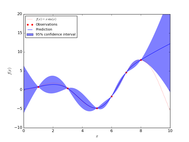
3) We fit our GPs to the data we observed. We know that the true function goes through these points because we observed them. What we don't know is how they are connected.


Not a great fit, but with only 2 observed data points, how could we do any better? Note that the red bands around the thick line is the uncertainty about the prediction. As you can see, the uncertainty around each observed data point is 0, because, well, we're certain that it goes through that point!
You can probably guess what happens as we observe more data points generated by this imaginary wave. But why guess?
There you have it! Using a basic Gaussian process, we're able to fit to our function with more and more accuracy as we get more data. So to recap:
- Some problems require us to use more flexible ML techniques, such as Gaussian Processes (GP)
- GPs are used widely in spatial statistics where there is a correlation between data points
- GPs don't care what the original function is that we're trying to estimate, which makes them non-parametric - generally a desired property of a model.
- GPs allow us to specify the covariance structure of our data - meaning that we can determine how we think the data are related. This leads to smooth curves vs. jagged ones.
- GPs allow us to quantify our uncertainty around our estimates.
- As we observe more data, our estimates become more certain.
If nothing else, think of this as your first step towards making it big in the stock market, now that you know a thing or two about how they are modeled. Or not.

